Scratch RecSys 01 - System Design and Scenario Framing for ZaPudia Recommendation Engine

About this Series

Let me introduce a dummy e-commerce for this Case, call as ZaPudia. Here is the scenario, it operates a dual-sided e-commerce marketplace in Indonesia at scale: 10 million registered users and 500,000 active SKUs spanning electronics, fashion, FMCG, and automotive verticals. Over the past two quarters, the platform’s personalization surface has degraded significantly. The legacy baseline, a zero-personalization, rule-based engine returning the global top-50 popular SKUs to all users, was simple, deterministic, inexpensive, and operationally reliable. However, it proved structurally incapable of capturing individual user intent. This reliance on global popularity triggered severe system-wide pathologies: extreme popularity bias, catalog rot, high cold-start failure rates for new merchants, and measurable churn among power users.

To quantifiably address this degradation, the engineering mandate targets the following metric trajectory:

Metric	Current Baseline	Strategic Target	Metric Scope / Business Impact
CTR	2.8%	4.2%+	+50% relative lift in item engagement
Conversion Rate (CVR)	2.4%	3.3%+	+37.5% relative lift in checkout conversion
Monthly ARPU	Baseline	+12%	Direct revenue expansion per active user
D30 Retention	Baseline	+8%	Long-term user lifetime value (LTV) growth
Cross-Sell Rate	Baseline	+15%	Enhanced catalog discovery across verticals
Session Depth	-18% vs. healthy	$\ge$ Baseline	Recovery of organic exploration depth
Recommendation P99	Unoptimized	< 100 ms	Strict online serving latency SLA

This series documents the end-to-end engineering journey of replacing the naive baseline with a scalable, multi-stage hybrid recommendation engine built around the cooprecsys library and a high-throughput ML serving stack, all while enforcing a strict sub-100 ms P99 latency SLA.

Part 1 establishes the architectural and mathematical foundation, delivering five core deliverables:

1. Forensic Business & Funnel Leakage Analysis: Unpacking where user intent drops off across the purchase funnel due to static recommendation surfaces.
2. Five Production Scenario Specifications: Complete architectural breakdowns (candidate generation, ranking strategy, and latency budget) for Homepage Feed, PDP Cross-Sell, Cold-Start Onboarding, Flash-Sale Intent, and Dormant User Re-engagement.
3. Visual System Architecture: An end-to-end event ingestion, offline batch training, and FastAPI serving pipeline, rendered using custom Astro React Flow components.
4. Rigorous Algorithm Derivations: Step-by-step mathematical formulations for Implicit Alternating Least Squares (iALS), Bayesian Personalized Ranking (BPR), and Two-Tower Softmax Cross-Entropy with in-batch negative sampling.
5. Decision Matrix & Offline-to-Online Selection Rules: A systematic framework mapping offline evaluation metrics (NDCG@K, Recall@K, MAP@K) to online business KPIs to prevent metric decoupling.

In this optimization framework, $\theta$ serves as the system configuration vector (or decision variable) that parameterizes the end-to-end recommendation pipeline. It encompasses model weights, serving parameters, such as candidate retrieval limits and caching rules and infrastructure resource allocations. By tuning $\theta$, the system maximizes business impact while strictly respecting the operational guardrails for latency, quality, reliability, and cost. In production recommender design, high accuracy without low latency is unusable, and low latency without personalization is useless. We frame the core production objective as a constrained multi-objective optimization problem:

$$\max_{\theta} \;\; \text{Business Impact}(\theta) \quad \cong \quad \begin{cases} \text{P99 Latency}(\theta) \le 100\text{ ms} \\ \\ \text{Recommendation Quality}(\theta) \ge Q_{\min} \\ \\ \text{System Reliability}(\theta) \ge 99.99\% \\ \\ \text{Infrastructure Cost}(\theta) \le C_{\max} \end{cases}$$

Subsequent installments will detail distributed offline training pipelines, feature store synchronization, real-time A/B testing infrastructure, and operational guardrails.

---

1. Business Context & Funnel Metric Leakage

1.1 The Dual-Sided Marketplace Failure Mode

Assume the ZaPudia platform is a marketplace, not a single-seller retailer. The health of the platform is a function of two interdependent populations: buyers (demand) and sellers (supply). A recommendation system that returns the same global top-50 SKUs to every user does not merely under-serve buyers it structurally damages both sides of the marketplace simultaneously.

$$\mathcal{U} = \{u_1,u_2,\ldots,u_m\}$$

The other side contains sellers and products:

$$\mathcal{I} = \{i_1,i_2,\ldots,i_n\}$$

with a seller-to-product mapping:

$$s(i) \rightarrow \text{seller of item } i$$

The recommendation layer therefore affects both sides simultaneously.

1.1.1 Buyer-Side Erosion (Demand Collapse)

When every user sees the same fifty SKUs, the personalization signal is zero. The consequences on the buyer side are compounding:

• Exploration starvation. Returning users with deep interaction history receive zero marginal utility from the feed the system has learned nothing about them. Power users, who account for a disproportionate share of GMV, see the same SKUs as first-time visitors and churn first.
• Session depth collapse. Without diversity or novelty, a user’s expected number of pages-per-session collapses to roughly “scan the homepage, leave.” The observed 17.6% session-depth drop is the empirical fingerprint of this effect.
• Cross-sell destruction. On the PDP, “Frequently Bought Together” surfaced from global co-occurrence returns the most co-purchased accessories in the catalog almost always a phone case and a screen protector which are irrelevant to a user browsing automotive parts. CTR on these modules erodes toward the noise floor.

1.1.2 Seller-Side Churn (Supply Collapse)

The supply-side damage is slower but more dangerous, because it is harder to detect and harder to reverse:

• New-seller cold-start death. A new seller listing a high-quality SKU enters a system where the only ranking signal is global popularity count. The SKU has zero historical interactions, so it can never accumulate interactions because it is never surfaced. This is a classic cold-start death spiral: no impressions $\to$ no clicks $\to$ no signal $\to$ no impressions.
• Long-tail catalog rot. With 500,000 active SKUs and only 50 ever surfaced, the impression share of the top decile approaches 100% while the long tail (the catalog’s genuine breadth) receives effectively zero traffic. SKUs that stop selling get delisted by sellers $\to$ catalog shrinks $\to$ marketplace differentiation vs. competitors erodes.
• Power-seller concentration risk. The same top-50 SKUs are dominated by a handful of power sellers. Concentrating GMV into a small seller cohort creates pricing power asymmetry and platform leverage risk; it also makes the marketplace brittle to a single large seller departing.

The fundamental architectural insight is that popularity bias is not a ranking problem to be tuned it is a structural failure of the candidate generation layer. A popularity baseline has a single candidate generator (global argmax over interaction counts) with no user conditioning. The fix is not a better scorer on top of the same candidates; the fix is a multi-stage pipeline with multiple user-conditioned candidate generators feeding a learned re-ranker.

1.2 Popularity Bias and the Self-Reinforcing Feedback Loop

In early-stage recommendation architectures, engineering teams frequently rely on a global popularity baseline as an initial production shortcut. Operationally, it is straightforward: aggregate historical user activity, rank items by global interaction count, and serve the top $N$ items across all recommendation surfaces. However, treating historical popularity as an unbiased proxy for user preference introduces a fundamental flaw in system dynamics. A naive popularity engine constantly confuses exposure opportunity with intrinsic item relevance.

The Naive Scoring Mechanism

Formally, consider a deterministic ranking function that calculates the score of item $i$ at time step $t$ purely based on its aggregated historical interaction metrics:

$$\text{Score}(i) = \text{Popularity}(i, t)$$

When this scoring function determines product placement, top-ranked items receive disproportionate visual real estate on the user’s viewport. In information retrieval and recommender system literature, this introduces severe position bias.

The observed probability of a user interacting with item $i$ is not merely a reflection of the item’s intrinsic utility $U(i)$, but rather a joint probability conditioned on exposure $E(i)$:

$$P(\text{Interaction} \mid i) = P(E(i) = 1) \cdot P(\text{Interaction} \mid E(i) = 1, U(i))$$

Because the static rule-based baseline forces top-ranked popular items to maintain $P(E(i) = 1) \approx 1$, these items accumulate massive impression volumes while long-tail items remain unexposed ($P(E(i_{\text{tail}}) = 1) \to 0$). Consequently, the observed click-through rate inflates artificially:

$$P(\text{Click} \mid \text{Impression}, i) \uparrow$$

The Interaction Cascade and Temporal Recurrence

Once an item gains exposure and secures an initial click, it initiates a downstream conversion cascade across the user journey:

$$\text{Click} \longrightarrow \text{Add-to-Cart} \longrightarrow \text{Checkout} \longrightarrow \text{Purchase}$$

These downstream events are logged by event streams and aggregated into offline batch tables, updating the item’s popularity state for the subsequent time window $t+1$:

$$\text{Popularity}(i, t+1) = \text{Popularity}(i, t) + \sum_{m \in M} w_m \cdot \Delta \text{Interaction}_m(i, t)$$

where $M = \{\text{click}, \text{add\_to\_cart}, \text{purchase}\}$ represents the set of interaction types, and $w_m$ denotes their respective weighting factors.

This update rule closes a positive feedback loop, a classical realization of preferential attachment (often referred to as the Matthew Effect, where high-performing items exponentially gain more traction):

$$\text{Popularity} \longrightarrow \text{Exposure} \longrightarrow \text{Interaction} \longrightarrow \text{Popularity}$$

Systemic Consequences: Catalog Rot and Marketplace Distortion

In a dual-sided marketplace like ZaPudia, housing 500,000 SKUs, this self-reinforcing loop severely distorts catalog distribution, creating three major operational failure modes:

• Catalog Rot: Over 95% of active SKUs never receive sufficient exposure to collect interaction signals. Items decay in search rank without ever being evaluated by users.
• Merchant Churn: New sellers face insurmountable cold-start barriers. Because their newly listed items have zero historical interactions, the baseline engine hides them, leading to merchant attrition.
• Power User Fatigue: High-intent repeat buyers are repeatedly exposed to static, generic top-sellers rather than personalized niche items, depressing D30 retention and long-term Customer Lifetime Value (LTV).

Core Engineering Takeaway
A naive recommender system does not merely measure historical popularity, it actively manufactures future popularity. Left uncorrected, the algorithm turns the recommendation surface into a self-fulfilling prophecy, replacing true personalization with self-generated exposure bias.

1.3 Catalog Rot and Long-Tail Starvation

Catalog rot is the structural outcome of prolonged popularity bias. In a healthy e-commerce ecosystem, product discovery follows a long-tail distribution where total aggregate volume across millions of niche items equals or exceeds the sales volume of blockbusters. When a recommender system relies solely on global popularity, it collapses this long tail into a rigid winner-take-all dynamic.

Formalizing the Exposure Allocation Failure

To quantify this phenomenon, let us formalize exposure and interaction metrics over an evaluation window $T$:

$$E_i = \sum_{t=1}^{T} \sum_{u \in U} \mathbb{I}(\text{Item } i \text{ exposed to User } u \text{ at time } t)$$ $$I_i = \sum_{t=1}^{T} \sum_{u \in U} \mathbb{I}(\text{User } u \text{ interacts with Item } i \text{ at time } t)$$

In a popularity-driven baseline, the exposure allocation mechanism creates a severe mathematical divergence between the top tier of popular SKUs and the remaining catalog:

$$E_{\text{top}} \gg E_{\text{long-tail}} \quad \text{where} \quad |\text{Top}| \ll |\text{Long-tail}|$$

This results in an extreme Pareto distribution where less than 1% of active SKUs capture over 90% of total system impressions ($E_{\text{top-50}} \approx \sum E_{\text{total}}$). The remaining 499,950 SKUs in ZaPudia’s catalog receive near-zero exposure ($E_{\text{long-tail}} \to 0$), rendering it mathematically impossible for the engine to evaluate their true interaction potential $I_{\text{long-tail}}$.

The Hidden Value Paradox of the Long Tail

The primary tragedy of catalog rot is not merely unexposed inventory, but the suppression of high-value inventory. Long-tail items frequently exhibit superior economic and strategic properties compared to mass-market items:

• Higher Profit Margins: Niche, specialized, or direct-to-consumer (D2C) items often carry higher gross margins than heavily discounted, price-competitive global bestsellers.
• Higher Satisfaction & Intent Alignment: When a user is matched with a specific, hard-to-find item fitting their exact parameters, conversion satisfaction and Net Promoter Score (NPS) peak.
• Low Merchant Competition: Long-tail SKUs diversify seller representation across the platform, preventing market monopolization by a handful of mega-distributors.
• Personalized Relevance: For specific user cohorts, long-tail relevance $P(i \mid u)$ vastly exceeds global baseline utility $P(i)$.

By starving the long tail of impressions ($E_{\text{long-tail}} \to 0$), the baseline engine prevents the platform from capturing the latent economic value of these high-margin SKUs, accelerating inventory decay and vendor dissatisfaction.

Popularity vs. Personalization

It is critical to distinguish between effective recommendation and global popularity filtering:

$$\text{Naive Recommender:} \quad P(\text{Item } i \mid \text{User } u) \approx P(\text{Item } i)$$ $$\text{Personalized Recommender:} \quad P(\text{Item } i \mid \text{User } u) = f(H_u, C_u, \theta_i)$$

where $H_u$ represents the historical context of user $u$, $C_u$ represents real-time session context, and $\theta_i$ denotes structural item embeddings.

Key Distinction
Popular products are not intrinsically bad recommendations; high global demand is a strong prior signal ($P(i)$). The structural failure occurs when a system treats global popularity as a complete substitute for personalized relevance, effectively reducing a complex personalized retrieval problem $P(i \mid u)$ to a static global ranking.

1.4 Power-User Churn and the Expectation Asymmetry

Recommender system performance cannot be evaluated uniformly across all user cohorts. A fundamental asymmetry exists between new or casual users and highly engaged power users. A cold-start user with zero historical footprint ($|H_u| \approx 0$) expects a degree of broad exploration, making them reasonably tolerant of a generic, globally popular surface. Conversely, power users, who drive a disproportionate share of platform GMV and high-margin transactions, demand precise, context-aware personalization that reflects their deep taste graph ($|H_u| \gg 0$).

Formalizing the Relevance Mismatch

Consider a power user $u$ with an established interaction history $H_u$ centered on high-intent niche verticals (e.g., custom mechanical keyboards, hot-swappable switches, GPU accessories, and enthusiast PC hardware). When the serving engine bypasses personal history and defaults to a static global popularity baseline $P(i)$, it introduces a massive utility discrepancy:

$$\text{Relevance}_{\text{global}}(i) = P(i) \;\ll\; P(i \mid H_u) = \text{Relevance}_{\text{personal}}(i)$$

Because $P(i)$ is dominated by mass-market, high-volume FMCG or fashion items, the probability that a globally popular product matches this power user’s specific intent approaches zero:

$$P(\text{Click} \mid \text{Global Top-50}, H_u) \to 0$$

The Attrition Cascade

When a power user repeatedly encounters irrelevance on high-value personalization surfaces (such as the homepage feed or product detail page recommendations), it triggers a progressive erosion of trust and engagement:

$$\text{Relevance Mismatch} \longrightarrow \text{Session Depth} \downarrow \; \longrightarrow \text{Order Frequency} \downarrow \; \longrightarrow \text{D30 Retention} \downarrow$$

1. Session Depth Decay: The user stops exploring recommended surfaces, reducing their session navigation depth ($\text{SessionDepth} \downarrow$).
2. Intent Relocation: Exploration shifts entirely to manual search queries, bypassing organic discovery.
3. Platform Churn: As friction increases, high-LTV users migrate to competitor platforms offering lower discovery friction, causing measurable retention drop-offs ($\text{Retention} \downarrow$).

System Design Imperative
Offline metrics like NDCG@K or Recall@K must be segmented by user activity tiers (e.g., Cold, Warm, Power User). Evaluating system performance solely on global averages hides critical power-user churn under high volume from casual clicks.

1.5 Dual-Sided Marketplace Dynamics: Buyer Erosion vs. Seller Churn

ZaPudia operates as a dual-sided marketplace. A naive recommendation architecture that optimizes exclusively for short-term buyer engagement metrics will destabilize the merchant ecosystem, causing severe long-term supply-side attrition.

Modeling Demand-Side Utility and Supply-Side Health

To build a sustainable marketplace engine, we must decouple and explicitly model both sides of the platform.

1. Demand-Side Buyer Value ($V_{\text{buyer}}$):
Measures immediate consumption utility and long-term user satisfaction across the purchase funnel:

$$V_{\text{buyer}} = f(\text{CTR}, \text{CVR}, \text{AOV}, \text{Retention}, \text{SessionDepth})$$

2. Supply-Side Ecosystem Health ($S_{\text{seller}}$):
Measures catalog distribution fairness, inventory mobility, and merchant retention:

$$S_{\text{seller}} = f(\text{ExposureFairness}, \text{InventoryVelocity}, \text{NewSKUExposure}, \text{GMV}_{\text{tail}})$$

The Hazard of Single-Metric Optimization

When an engineering team configures the ranking objective strictly to maximize immediate buyer click-through rate ($\max \text{CTR}$), the model optimizes for short-term engagement proxies. It exploits items with high baseline clickability while ignoring catalog distribution dynamics. This short-sighted optimization leads to a severe systemic failure mode:

$$\begin{cases} \text{Buyer CTR} \uparrow \\ \text{Catalog Coverage} \downarrow \\ \text{Seller Churn} \uparrow \end{cases}$$

In this regime, fewer than 1% of merchants capture virtually all recommendation traffic. Long-tail sellers, unable to secure baseline impressions for new inventory, face inventory stagnation and high platform exit rates ($\text{SellerChurn} \uparrow$).

Over time, seller attrition degrades catalog diversity, which ultimately turns back to destroy buyer value ($V_{\text{buyer}} \downarrow$).

The Multi-Objective Ranking Mandate

To mitigate dual-sided collapse, modern production scoring functions must be framed as a Multi-Objective Optimization (MOO) problem. The final ranking score $S(u, i)$ for user $u$ and item $i$ must explicitly balance buyer intent, item economics, and supply-side health constraints:

$$S(u, i) = w_1 \cdot P(\text{Click} \mid u, i) + w_2 \cdot P(\text{Conversion} \mid u, i) + w_3 \cdot \text{Margin}(i) + w_4 \cdot \Omega_{\text{fairness}}(i)$$

where $\Omega_{\text{fairness}}(i)$ acts as a dynamic exploration boost for new or under-exposed SKUs, ensuring that the recommendation engine actively balances buyer conversion with supply-side merchant retention.

1.6 Baseline vs. Target KPI Matrix

The engineering mandate establishes explicit target KPIs. The table below is the contractual reference for every architectural decision that follows: if a design choice does not move these numbers, it is out of scope.

Metric	Definition	Baseline (Current)	Target (12-Week)	Target (Q4)	Delta vs. Baseline
CTR	Ratio of clicks to impressions across recommendation surfaces	2.8%	3.6%	4.4%	+57%
CVR	Ratio of orders to sessions with $\ge 1$ recommendation impression	2.4%	3.0%	3.6%	+50%
Monthly ARPU	Ratio of Gross Merchandise Value (GMV) to active users per month	IDR 312k	IDR 385k	IDR 450k	+44%
D30 Retention	Percentage of cohort active on Day 30 post-first session	11.2%	14.5%	18.0%	+61%
Cross-Sell Rate	Percentage of orders containing $\ge 2$ distinct product categories	8.4%	13.0%	18.0%	+114%
Session Depth	Average number of page views per session	5.6	6.8	7.4	+32%
Catalog Coverage	Ratio of daily unique SKUs surfaced to total active catalog	0.01%	8%	25%
P99 Serving Latency	99th percentile end-to-end recommendation response time	N/A (cache)	$\le 100\text{ ms}$	$\le 80\text{ ms}$

The Catalog Coverage target is the most architecturally revealing: moving from 0.01% (50 SKUs of 500k) to 25% (125,000 SKUs surfaced per day) is impossible with a single candidate generator. It is the single strongest argument for the multi-stage architecture in Section 3.

1.7 Revenue Leakage Across the Interaction Funnel

The user interaction funnel for a recommendation surface decomposes into four stages. The table quantifies per-stage leakage using the observed deltas, expressed in terms of lost conversion opportunities per 1 million recommendation impressions.

Funnel Stage	Healthy Conv. (per 1M imp.)	Current Conv. (per 1M imp.)	Leakage Volume	Estimated GMV Leakage / day (IDR)
Impression $\to$ Click (CTR)	41,000 clicks	28,000 clicks	13,000 lost clicks	13,000 × 0.084 CVR² × IDR 185k AOV $\approx$ 202M
Click $\to$ Cart-Add (ATC rate)	14,350 (35% of clicks)	8,400 (30% of clicks)	5,950 lost cart-adds	5,950 × 0.245 × 185k $\approx$ 270M
Cart-Add $\to$ Checkout	10,043 (70%)	5,880 (70%)	4,163 lost checkouts	4,163 × 185k $\approx$ 770M
Checkout $\to$ Order (CVR)	8,035 (80%)	4,234 (72%)	3,801 lost orders	3,801 × 185k $\approx$ 703M

Note: figures are illustrative decomposition using representative sub-funnel rates; the structure not the absolute numbers is the design-relevant output. The aggregate finding is that the largest recoverable leakage is in the upper funnel (Impression $\to$ Click), which is precisely the surface a re-ranker most directly controls.

The architectural consequence is direct: the re-ranking layer owns the Impression $\to$ Click transition, the candidate generation layer owns coverage and cold-start (Cart-Add and Checkout volume depend on surfacing relevant-but-unseen SKUs), and the serving layer owns the latency budget that prevents upper-funnel abandonment from slow loads. Section 2 allocates these responsibilities across five concrete scenarios.

---

2. The 5 Specific ZaPudia Scenarios

A multi-stage recommender isn’t just one monolithic model doing all the heavy lifting; it’s more like a portfolio of scenario-specific pipelines that all leverage the same core infrastructure, like our feature store, candidate index, and serving layer. To make sure every use case gets what it needs, each scenario is explicitly broken down by its Business Goal, Input Telemetry, Candidate Generation Strategy, Ranking Method, and Target Latency Budget. Thinking of these specifications as architectural contracts helps bridge the gap between business needs and system design, directly setting the technical benchmarks that our Section 3 architecture has to satisfy.

2.1 Scenario A Homepage Feed Personalization

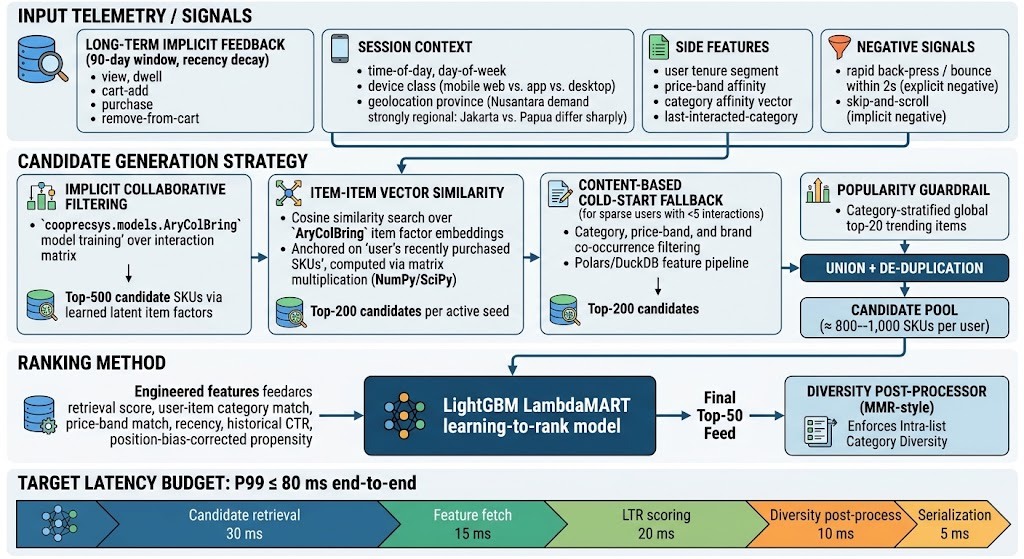
Business Goal. Maximize discovery and session depth for returning users on the homepage feed. This is the highest-volume surface ($\approx$ 62% of all recommendation impressions) and the primary driver of the CTR and session-depth targets. The objective is broad ranking over implicit feedback, the user has not stated an intent; we must infer it from history and rank the full candidate pool accordingly.

Input Telemetry / Signals.

• Long-term implicit feedback: view, dwell, cart-add, purchase, remove-from-cart events over a 90-day window, weighted by recency decay.
• Session context: time-of-day, day-of-week, device class (mobile web vs. app vs. desktop), geolocation province (Nusantara demand is strongly regional Jakarta vs. Papua differ sharply).
• Side features: user tenure segment, price-band affinity, category affinity vector, last-interacted-category.
• Negative signals: rapid back-press / bounce within 2s treated as explicit negative; skip-and-scroll as implicit negative.

Candidate Generation Strategy. Multi-generator union with de-duplication:

1. Implicit Collaborative Filtering: cooprecsys.models.AryColBring model training over the implicit interaction matrix, retrieving top-500 candidate SKUs per user via learned latent item factors.
2. Item-Item Vector Similarity: Cosine similarity search over AryColBring item factor embeddings anchored on the user’s recently purchased SKUs (top-200 candidates per active seed), computed via matrix multiplication (NumPy/SciPy).
3. Content-Based Cold-Start Fallback: Category, price-band, and brand co-occurrence filtering (via Polars/DuckDB feature pipeline) generating top-200 candidates for sparse users with $< 5$ historical interactions.
4. Popularity Guardrail: Category-stratified global top-20 trending items to guarantee a coverage floor and prevent cold-item starvation without over-indexing bias.

Union + de-duplication $\to$ candidate pool of $\approx 800\text{--}1.000$ SKUs per user.

Ranking Method. A LightGBM LambdaMART learning-to-rank model over engineered features (retrieval score, user-item category match, price-band match, recency, historical CTR of the item, position-bias-corrected propensity). The re-ranker produces the final top-50 feed. A diversity post-processor (MMR-style, see §4.3 ILD) enforces intra-list category diversity to prevent a single category dominating the feed.

Target Latency Budget. P99 $\le$ 80 ms end-to-end (homepage is on the critical render path). Allocation: candidate retrieval 30 ms · feature fetch 15 ms · LTR scoring 20 ms · diversity post-process 10 ms · serialization 5 ms.

2.2 Scenario B Product Detail Page (PDP) “Frequently Bought Together”

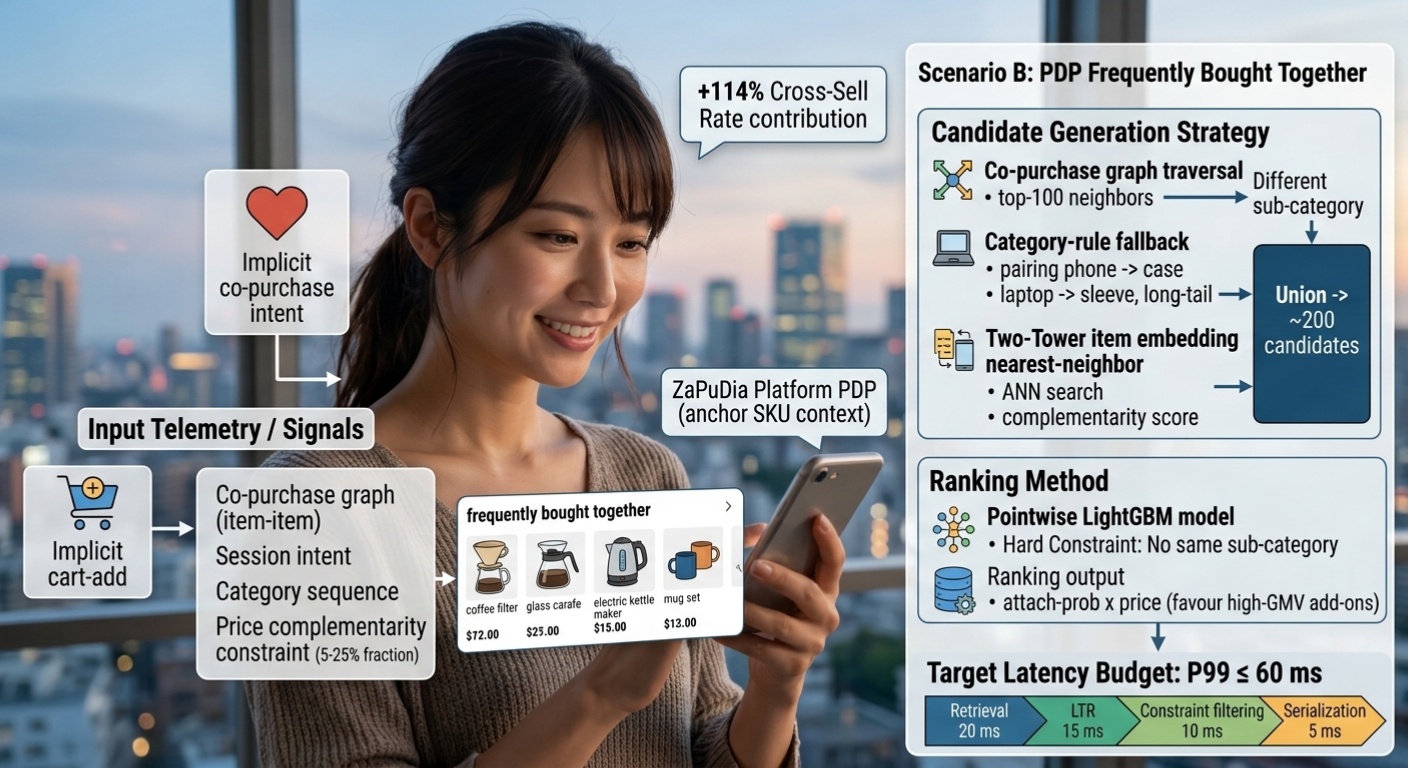
Business Goal. Drive cross-sell by surfacing complementary SKUs (not substitutes) on the PDP. The success metric is the Cross-Sell Rate (orders containing $\ge 2$ distinct categories) and add-on attach rate. This scenario is the single largest contributor to the Cross-Sell Rate target (+114%).

Input Telemetry / Signals.

• The anchor SKU context: category, sub-category, price, brand, attributes.
• User co-purchase graph: item-item co-occurrence within the same order (not same-session, co-purchase is a stronger complementarity signal than co-view).
• Session intent: current session’s category sequence (did the user arrive from a search for “laptop” or “gift”?).
• Price complementarity constraint: complementary items should sit in a different but related category and a price band that is a fraction (typically 5–25%) of the anchor’s price.

Candidate Generation Strategy.

1. Co-purchase graph traversal (the model will trained on the binary co-purchase matrix, Jaccard similarity) top-100 neighbors of the anchor SKU restricted to different sub-category (to enforce complementarity over substitutability).
2. Category-rule fallback deterministic category pairing rules (phone $\to$ case, laptop $\to$ sleeve, motorcycle $\to$ helmet) for the long-tail anchor SKUs with sparse co-purchase data.
3. Two-Tower item embedding nearest-neighbor ANN search over the item tower’s embedding space, filtered to top-50 by complementarity score. Union $\to \approx 200$ candidates.

Ranking Method. A pointwise LightGBM model optimized for attach probability (P(add-to-cart | anchor in cart)) with a hard constraint: no item from the same sub-category as the anchor may appear. The top-4 are returned, sorted by attach-prob × price (to favor high-GMV add-ons).

Target Latency Budget. P99 $\le 60$ ms (PDP module loads after hero content). Allocation: retrieval 20 ms · LTR 15 ms · constraint filtering 10 ms · serialization 5 ms. PDP candidates may be edge-cached per anchor SKU with a 1-hour TTL, since the anchor context is static; only the user-conditional re-rank is computed live.

2.3 Scenario C Cold-Start Strategy (New Users & Unrated SKUs)

Business Goal. Eliminate the cold-start death spiral identified in §1.1.2. Two distinct cold-start problems are solved by one strategy: new users (no interaction history) and new/unrated SKUs (no interaction signal). The objective is a graceful degradation curve: a new user or new SKU should perform no worse than the popularity baseline on day 1 and improve monotonically as signal accrues.

Input Telemetry / Signals.

• New user : registration attributes (province, age band declared, acquisition channel), first-session implicit signals (first 3 clicks within 60s available even in the first session).
• New SKU : seller-provided metadata (category, brand, price, attributes, images $\to$ CLIP embedding), seller’s historical performance (the seller’s prior SKUs’ average CTR/CVR as a prior).
• Side-feature fallback : category × province popularity, price-band × province popularity.

Candidate Generation Strategy.

• New users: hybrid routing
  1. If province + age band is known $\to$ segment-popular (top-K within the segment) provides the floor.
  2. First-session clicks trigger an online item-item similarity expansion from the clicked SKU’s item-factors (available immediately, no retraining needed).
  3. After 5 interactions, switch to the full iALS user-factor path.
• New SKUs: zero-shot scoring via content-based embedding (CLIP image embedding + text attributes) projected into the item-factor space via a learned linear mapping; popularity prior seeded from the seller’s portfolio. The SKU is eligible for the popularity-guardrail slot until it accumulates $\ge 50$ impressions, at which point it graduates to the iALS candidate pool.

Ranking Method. A calibrated blending of content-based score and popularity-prior score, blended with weight w that decays as interaction count grows: $\text{score}(u, i) = w(n_u) \cdot \text{score}_{\text{pop}}(i) + (1 - w(n_u)) \cdot \text{score}_{\text{cb}}(u, i), \quad w(n_u) = e^{-n_u / \tau_c}$ where $n_u$ is the user’s interaction count and $\tau_c$ is a confidence half-life (tuned, typically 10). The blend guarantees monotonic improvement: at $n_u = 0$ it is pure popularity; as $n_u \to \infty$ it is pure personalization.

Target Latency Budget. P99 $\le 100$ ms (no harder than homepage; the cold-start path shares the homepage retrieval budget but uses a different scorer).

2.4 Scenario D Flash Sale & Real-Time Session Intent

Business Goal. Capture short-term preference shifts during hourly flash-sale windows. During a flash sale, user intent changes within minutes, a user who normally browses fashion may pivot hard to electronics during a noon electronics flash sale. The static iALS factors (trained daily) cannot represent this; the pipeline must incorporate a real-time session signal with sub-minute freshness.

Input Telemetry / Signals.

• Real-time session events via Kafka stream: last 10 events in the current session with sub-second latency.
• Flash-sale catalog manifest: the set of sale SKUs, their discount depth, and the sale window [start, end].
• Time-in-window: minutes elapsed since sale start (early-window users browse more broadly; late-window users convert faster).
• Inventory pressure: remaining stock / initial stock (urgency signal).

Candidate Generation Strategy.

1. Session-item similarity over a session-conditioned item embedding (a lightweight session tower updated every 5 minutes) $\to$ top-200.
2. Flash-sale catalog injection the sale SKUs are force-included as candidates but never force-ranked; they compete in the re-ranker with an urgency-prior boost.
3. iALS long-term candidates top-200 from the daily-trained factors, to preserve personalization for users whose session intent has not shifted. Union $\to \approx 600$ candidates.

Ranking Method. A session-aware neural re-ranker (a small 2-layer MLP over [session embedding, item embedding, long-term user factor, sale features]) trained on logged-bandit data from prior flash sales. The urgency prior is added as an additive log-odds shift on the flash-sale candidates, bounded to prevent sale items from dominating non-sale users.

Target Latency Budget. P99 $\le$ 50 ms (flash-sale users are high-intent and latency-sensitive; any delay risks losing the sale to a competitor). This is achieved by keeping the session tower tiny (32-dim) and precomputing the session-item ANN index. Allocation: session-embedding fetch 10 ms · retrieval 15 ms · neural re-rank 15 ms · serialization 10 ms.

2.5 Scenario E Batch Push Notification & Re-engagement (Dormant > 14 Days)

Business Goal. Reactivate dormant users (last active > 14 days) via personalized push notifications containing 1–3 recommended SKUs. This is an offline, batch scenario, there is no latency SLA on the user-facing path; the constraint is throughput and the quality-per-impression cost of a push (push notifications have a strict fatigue budget: a bad recommendation causes an unsubscription, which is far costlier than a bad homepage impression).

Input Telemetry / Signals.

• Full 180-day interaction history (longer horizon than homepage; dormant users need richer context to be reactivated).
• Last-active category and last-abandoned-cart SKUs (the strongest reactivation signal a user who abandoned a cart is high-intent).
• Lifecycle segment: lapsed-buyer (previously purchased), browser-only (never purchased), churned-power-user (high historical GMV, now dormant).

Candidate Generation Strategy. Batch pre-computed overnight:

1. iALS full retrain on the 180-day matrix $\to$ top-200 per user.
2. Abandoned-cart recovery SKUs in the user’s last abandoned cart, deduped against purchased.
3. New-arrival personalization SKUs listed in the last 14 days (since the user was last active) that match the user’s category affinity (the “you missed these” hook).
4. Lifecycle-segment popular for browser-only users with no purchase history, segment-popular provides the floor. Union $\to \approx 400$ candidates.

Ranking Method. A two-stage ranker: (1) LightGBM predicted open-probability × predicted post-open conversion-probability (the value of a push is open × convert, not just click); (2) a fatigue/ unsubscription-risk penalty modeled as a logistic regression over prior 30-day push frequency. The final score is: $\text{push\_score}(u, i) = P(\text{open} \mid u, i) \cdot P(\text{convert} \mid \text{open}, u, i) - \lambda_{\text{fatigue}} \cdot P(\text{unsub} \mid u, \text{recent pushes})$

Target Latency Budget. No user-facing SLA (batch). Throughput SLA: full scoring of the dormant cohort (typically 1.5–2 M users) within a 4-hour overnight window on the training cluster. The serving-side SLA is only the push-scheduler lookup: P99 $\le 30$ ms for a single user’s pre-computed recommendations from Redis.

2.6 Scenario Summary Matrix

Scenario	Surface	Freshness	Primary Generator	Ranker	P99 Latency
A · Homepage Feed	Home	Daily + session	iALS + ItemKNN + Content	LightGBM LTR + MMR	$\le$ 80 ms
B · PDP FBT	PDP	Hourly (cached)	Co-purchase KNN + Two-Tower	LightGBM attach	$\le$ 60 ms
C · Cold-Start	All surfaces	Real-time	Segment-pop + Content + Online KNN	Calibrated blend	$\le$ 100 ms
D · Flash Sale	Home / Sale hub	Sub-minute	Session-tower KNN + iALS	Neural re-ranker	$\le$ 50 ms
E · Push Re-engagement	Push (batch)	Daily batch	iALS (180d) + Cart + New-arrivals	2-stage value − fatigue	N/A (batch)

---

3. Visual System Architecture (Astro React Flow Integration)

3.1 End-to-End Multi-Stage Pipeline (Primary Canvas)

Reading the diagram (left $\to$ right):

1. Ingestion lane, Kafka + GA4 + App SDK produce raw events; the Avro/Protobuf schema registry guarantees contract stability between producers and the stream processor.
2. Feature lane, Flink/Spark Streaming materializes three stores in parallel: the online feature store (Redis), the implicit interaction matrix (DuckDB for offline batch, Redis for online lookup), and the sub-second session context store.
3. Training lane, A nightly batch job trains iALS/BPR/Two-Tower over the interaction matrix; the LTR model is trained on logged-bandit labels joined with session context. Both publish artifacts to the MLflow/S3 model store.
4. Retrieval lane, At request time, model from Cooprecsys candidate generators (AryColBring/ALS) and the ScaNN/FAISS ANN index over Two-Tower item embeddings each produce a candidate stream; the cold-start guardrail guarantees a coverage floor.
5. Rerank + serve lane, Candidates are unioned and de-duplicated, scored by the LightGBM LTR re-ranker enriched with online features, post-processed for diversity, and served by the async FastAPI layer with edge caching on the client path.

3.2 Latency Budget Decomposition (Secondary Canvas)

This canvas isolates the P99 latency budget for the homepage (Scenario A) path, the most latency-critical surface, showing how the 80 ms budget is partitioned across stages. The edge labels are the millisecond allocations.

The critical observation is that retrieval (30 ms) and re-ranking (20 ms) together consume 62.5% of the budget. Both are parallelizable: the three candidate generators run concurrently (max-of-three latency, not sum), and the LTR scoring is a single batched LightGBM predict over the merged candidate set. The FastAPI layer must be async with non-blocking I/O on every Redis/ANN call to hold the budget.

---

4. Step-by-Step Mathematical Formulations & Proofs

This section provides the full mathematical derivations for the three core algorithms underpinning the ZaPudia architecture. Every reduction is shown explicitly; no step is elided.

4.1 Implicit Alternating Least Squares (iALS)

4.1.1 Setup and Notation

Let $m$ be the number of users and $n$ the number of items. The implicit feedback matrix $\mathbf{R} \in \mathbb{R}^{m \times n}$ contains raw interaction strengths (view counts, dwell-weighted events). We do not treat unobserved entries as true negatives; instead we introduce:

• Preference $p_{ui} \in \{0, 1\}$: $p_{ui} = 1$ if $R_{ui} > 0$ (user $u$ interacted with item $i$), and $p_{ui} = 0$ otherwise.
• Confidence $c_{ui} = 1 + \alpha R_{ui}$, with $\alpha > 0$ a confidence-scaling hyperparameter. The constant $+1$ gives every user-item pair a baseline confidence of 1, and confidence grows linearly with observed interaction strength.

We seek low-rank user and item factor matrices:

$\mathbf{U} = [\mathbf{u}_1, \dots, \mathbf{u}_m]^T \in \mathbb{R}^{m \times k}, \qquad \mathbf{V} = [\mathbf{v}_1, \dots, \mathbf{v}_n]^T \in \mathbb{R}^{n \times k}$

with latent dimension $k \ll \min(m, n)$. The predicted preference is $\hat{p}_{ui} = \mathbf{u}_u^T \mathbf{v}_i$.

4.1.2 Objective Function

$\mathcal{L}_{\text{iALS}} = \sum_{u=1}^{m} \sum_{i=1}^{n} c_{ui} \left( p_{ui} - \mathbf{u}_u^T \mathbf{v}_i \right)^2 + \lambda \left( \sum_{u=1}^{m} \|\mathbf{u}_u\|_2^2 + \sum_{i=1}^{n} \|\mathbf{v}_i\|_2^2 \right)$

The first term is a confidence-weighted squared reconstruction error over all $m \times n$ user-item pairs (including the unobserved ones, with $p_{ui} = 0$ and $c_{ui} = 1$); the second is L2 regularization preventing factor norm inflation.

4.1.3 Derivation of the Closed-Form User Update

We derive $\frac{\partial \mathcal{L}}{\partial \mathbf{u}_u} = 0$ while holding $\mathbf{V}$ (and hence all $\mathbf{v}_i$) fixed. Isolate the terms in $\mathcal{L}$ that depend on $\mathbf{u}_u$:

$\mathcal{L}_u = \sum_{i=1}^{n} c_{ui} \left( p_{ui} - \mathbf{u}_u^T \mathbf{v}_i \right)^2 + \lambda \|\mathbf{u}_u\|_2^2$

Step 1, Expand the squared term. Let $\hat{p}_{ui} = \mathbf{u}_u^T \mathbf{v}_i$.

$\left( p_{ui} - \mathbf{u}_u^T \mathbf{v}_i \right)^2 = p_{ui}^2 - 2 p_{ui} \, \mathbf{u}_u^T \mathbf{v}_i + \left( \mathbf{u}_u^T \mathbf{v}_i \right)^2$

Step 2, Differentiate w.r.t. $\mathbf{u}_u$. Using $\frac{\partial}{\partial \mathbf{u}_u} (\mathbf{u}_u^T \mathbf{v}_i) = \mathbf{v}_i$ and $\frac{\partial}{\partial \mathbf{u}_u} (\mathbf{u}_u^T \mathbf{v}_i)^2 = 2 (\mathbf{u}_u^T \mathbf{v}_i) \mathbf{v}_i$:

$\frac{\partial}{\partial \mathbf{u}_u} \left( p_{ui} - \mathbf{u}_u^T \mathbf{v}_i \right)^2 = -2 p_{ui} \mathbf{v}_i + 2 (\mathbf{u}_u^T \mathbf{v}_i) \mathbf{v}_i = -2 (p_{ui} - \mathbf{u}_u^T \mathbf{v}_i) \mathbf{v}_i$

Step 3, Assemble the full derivative. Including the regularization term $\frac{\partial}{\partial \mathbf{u}_u} \lambda \|\mathbf{u}_u\|_2^2 = 2 \lambda \mathbf{u}_u$:

$\frac{\partial \mathcal{L}_u}{\partial \mathbf{u}_u} = \sum_{i=1}^{n} c_{ui} \left[ -2 (p_{ui} - \mathbf{u}_u^T \mathbf{v}_i) \mathbf{v}_i \right] + 2 \lambda \mathbf{u}_u = \mathbf{0}$

Step 4, Factor out and simplify. Divide by $-2$:

$\sum_{i=1}^{n} c_{ui} (p_{ui} - \mathbf{u}_u^T \mathbf{v}_i) \mathbf{v}_i - \lambda \mathbf{u}_u = \mathbf{0}$

Expand the sum:

$\sum_{i=1}^{n} c_{ui} \, p_{ui} \, \mathbf{v}_i - \sum_{i=1}^{n} c_{ui} (\mathbf{u}_u^T \mathbf{v}_i) \mathbf{v}_i - \lambda \mathbf{u}_u = \mathbf{0}$

Step 5, Vectorize. Define the diagonal confidence matrix for user $u$:

$\mathbf{C}^u = \operatorname{diag}(c_{u1}, c_{u2}, \dots, c_{un}) \in \mathbb{R}^{n \times n}$

the preference vector $\mathbf{p}(u) = [p_{u1}, \dots, p_{un}]^T \in \mathbb{R}^{n}$, and recall $\mathbf{V} \in \mathbb{R}^{n \times k}$ stacks item factors as rows. Then:

• $\displaystyle \sum_{i=1}^{n} c_{ui} \, p_{ui} \, \mathbf{v}_i = \mathbf{V}^T \mathbf{C}^u \mathbf{p}(u)$
• $\displaystyle \sum_{i=1}^{n} c_{ui} (\mathbf{u}_u^T \mathbf{v}_i) \mathbf{v}_i = \sum_{i=1}^{n} c_{ui} \mathbf{v}_i \mathbf{v}_i^T \mathbf{u}_u = \mathbf{V}^T \mathbf{C}^u \mathbf{V} \, \mathbf{u}_u$

where we used $\mathbf{u}_u^T \mathbf{v}_i = \mathbf{v}_i^T \mathbf{u}_u$ (scalars commute) and the outer-product identity $\mathbf{v}_i \mathbf{v}_i^T$.

Step 6, Substitute and solve. The stationarity condition becomes:

$\mathbf{V}^T \mathbf{C}^u \mathbf{p}(u) - \mathbf{V}^T \mathbf{C}^u \mathbf{V} \, \mathbf{u}_u - \lambda \mathbf{u}_u = \mathbf{0}$

Group the $\mathbf{u}_u$ terms:

$\left( \mathbf{V}^T \mathbf{C}^u \mathbf{V} + \lambda \mathbf{I}_k \right) \mathbf{u}_u = \mathbf{V}^T \mathbf{C}^u \mathbf{p}(u)$

Hence the closed-form user update:

$\boxed{\; \mathbf{u}_u = \left( \mathbf{V}^T \mathbf{C}^u \mathbf{V} + \lambda \mathbf{I}_k \right)^{-1} \mathbf{V}^T \mathbf{C}^u \mathbf{p}(u) \;}$

The item update is symmetric, obtained by holding $\mathbf{U}$ fixed and repeating the derivation with $\mathbf{u} \leftrightarrow \mathbf{v}$:

$\mathbf{v}_i = \left( \mathbf{U}^T \mathbf{C}^i \mathbf{U} + \lambda \mathbf{I}_k \right)^{-1} \mathbf{U}^T \mathbf{C}^i \mathbf{p}(i)$

where $\mathbf{C}^i = \operatorname{diag}(c_{1i}, \dots, c_{mi}) \in \mathbb{R}^{m \times m}$ and $\mathbf{p}(i) \in \mathbb{R}^{m}$.

4.1.4 Matrix Dimensions and the Computational Bottleneck

Symbol	Shape	Meaning
$\mathbf{V}$	$n \times k$	item factor matrix (fixed during user update)
$\mathbf{C}^u$	$n \times n$	diagonal per-user confidence matrix
$\mathbf{V}^T \mathbf{C}^u \mathbf{V}$	$k \times k$	the Gram matrix to invert
$\mathbf{p}(u)$	$n \times 1$	per-user preference vector
$\mathbf{u}_u$	$k \times 1$	updated user factor

The bottleneck. A naive formation of $\mathbf{V}^T \mathbf{C}^u \mathbf{V}$ costs $O(n k^2)$ per user and materializes an $n \times n$ dense matrix if implemented literally as $\mathbf{C}^u \mathbf{V}$ first. With $n = 500{,}000$ and $k = 64$, the literal computation is $O(500{,}000 \times 64^2) \approx 2 \times 10^9$ flops per user, infeasible across $10^7$ users.

Mitigation 1, exploit the diagonal structure of $\mathbf{C}^u$. Because $\mathbf{C}^u$ is diagonal, $\mathbf{C}^u \mathbf{V}$ is just row-scaling of $\mathbf{V}$ by $c_{ui}$; no $n \times n$ matrix is ever materialized. The Gram matrix becomes:

$\mathbf{V}^T \mathbf{C}^u \mathbf{V} = \sum_{i=1}^{n} c_{ui} \, \mathbf{v}_i \mathbf{v}_i^T$

a sum of $n$ rank-1 $k \times k$ outer products, computed in $O(n k^2)$ with $O(k^2)$ memory. The inversion is $O(k^3)$, negligible for small $k$.

Mitigation 2, exploit confidence sparsity. Write $c_{ui} = 1 + \alpha R_{ui}$. Then:

$\mathbf{V}^T \mathbf{C}^u \mathbf{V} = \mathbf{V}^T \mathbf{V} + \alpha \sum_{i \in \mathcal{I}_u} R_{ui} \, \mathbf{v}_i \mathbf{v}_i^T$

where $\mathcal{I}_u = \{i : R_{ui} > 0\}$ is the (small) set of items user $u$ interacted with. The term $\mathbf{V}^T \mathbf{V}$ is user-independent and computed once per iteration; the second sum ranges only over $|\mathcal{I}_u| \ll n$ items. This is the Hu-Koren-Volinsky CG optimization: per-user cost drops from $O(n k^2)$ to $O(|\mathcal{I}_u| k^2 + k^3)$.

Mitigation 3, Woodbury / conjugate gradient. For very large $k$, the $k \times k$ solve can be replaced by conjugate gradient on the system $(\mathbf{V}^T \mathbf{C}^u \mathbf{V} + \lambda \mathbf{I}) \mathbf{u}_u = \mathbf{V}^T \mathbf{C}^u \mathbf{p}(u)$, using only matrix-vector products with $\mathbf{V}^T \mathbf{C}^u \mathbf{V}$ (no explicit inversion). This is the basis of the cooprecsys iALS solver’s scalable path for $k \geq 256$.

4.2 Bayesian Personalized Ranking (BPR) Loss

4.2.1 Pairwise Preference Setup

BPR optimizes relative preference rather than absolute reconstruction. For each user $u$, we observe a set of positive items $\mathcal{I}_u^+$ (interacted) and the complement $\mathcal{I} \setminus \mathcal{I}_u^+$ (non-interacted). For a sampled triple $(u, i^+, i^-)$ with $i^+ \in \mathcal{I}_u^+$, $i^- \notin \mathcal{I}_u^+$, we model the latent pairwise preference:

$i^+ >_u i^- \quad \Longleftrightarrow \quad \hat{x}_{u i^+} - \hat{x}_{u i^-} > 0$

where $\hat{x}_{ui} = \mathbf{u}_u^T \mathbf{v}_i$ is the model’s predicted score. The probability that $u$ prefers $i^+$ over $i^-$ is modeled by the sigmoid of the score difference:

$P(i^+ >_u i^- \mid \Theta) = \sigma\left( \hat{x}_{u i^+} - \hat{x}_{u i^-} \right), \qquad \sigma(z) = \frac{1}{1 + e^{-z}}$

Here $\Theta = \{\mathbf{U}, \mathbf{V}\}$ denotes all model parameters.

4.2.2 MAP Objective via Bayesian Posterior

Assuming independent triples and a Gaussian prior $\Theta \sim \mathcal{N}(\mathbf{0}, \lambda_\Theta^{-1} \mathbf{I})$, the Maximum A Posteriori objective is the negative log-posterior:

$\mathcal{L}_{\text{BPR}} = -\sum_{(u, i^+, i^-)} \ln \sigma\left(\hat{x}_{u i^+} - \hat{x}_{u i^-}\right) + \lambda_\Theta \|\Theta\|^2$

The first term is the negative log-likelihood of the observed pairwise preferences; the second is the negative log-prior (L2 regularization with strength $\lambda_\Theta$).

4.2.3 Derivation of the Parameter Gradient

Let $\theta \in \Theta$ be a single parameter (e.g., one entry of $\mathbf{u}_u$ or $\mathbf{v}_i$). Define the per-triple loss:

$\ell(u, i^+, i^-) = -\ln \sigma\left( \hat{x}_{u i^+} - \hat{x}_{u i^-} \right) + \frac{\lambda_\Theta}{|\mathcal{T}|} \|\Theta\|^2$

where $\mathcal{T}$ is the set of sampled triples (the regularization is amortized over the batch).

Step 1, Differentiate the log-sigmoid term. Let $z = \hat{x}_{u i^+} - \hat{x}_{u i^-}$. Using $\frac{d}{dz} \ln \sigma(z) = 1 - \sigma(z)$:

$\frac{\partial}{\partial \theta} \left[ -\ln \sigma(z) \right] = -(1 - \sigma(z)) \cdot \frac{\partial z}{\partial \theta} = -(1 - \sigma(z)) \left( \frac{\partial \hat{x}_{u i^+}}{\partial \theta} - \frac{\partial \hat{x}_{u i^-}}{\partial \theta} \right)$

Step 2, Add the regularization derivative. $\frac{\partial}{\partial \theta} \lambda_\Theta \|\Theta\|^2 = 2 \lambda_\Theta \, \theta$ (absorbing the factor of 2 into the conventional $\lambda_\Theta$ definition).

Step 3, Assemble the gradient. Let $\hat{\sigma} = \sigma(\hat{x}_{u i^+} - \hat{x}_{u i^-})$ for brevity. Then:

$\boxed{\; \frac{\partial \mathcal{L}_{\text{BPR}}}{\partial \theta} = \sum_{(u, i^+, i^-)} \left[ -(\hat{\sigma} - 1) \left( \frac{\partial \hat{x}_{u i^+}}{\partial \theta} - \frac{\partial \hat{x}_{u i^-}}{\partial \theta} \right) \right] + \lambda_\Theta \, \theta \;}$

Equivalently, using the common sign convention $\hat{\sigma} - 1 = -(1 - \hat{\sigma})$:

$\frac{\partial \mathcal{L}_{\text{BPR}}}{\partial \theta} = \sum_{(u, i^+, i^-)} (1 - \hat{\sigma}) \left( \frac{\partial \hat{x}_{u i^+}}{\partial \theta} - \frac{\partial \hat{x}_{u i^-}}{\partial \theta} \right) + \lambda_\Theta \, \theta$

Step 4, Resolve the score derivatives per parameter.

• For a user factor entry $\theta = u_{uf}$ (the $f$-th component of $\mathbf{u}_u$): since $\hat{x}_{ui} = \mathbf{u}_u^T \mathbf{v}_i = \sum_f u_{uf} v_{if}$, $\frac{\partial \hat{x}_{u i^+}}{\partial u_{uf}} = v_{i^+ f}, \qquad \frac{\partial \hat{x}_{u i^-}}{\partial u_{uf}} = v_{i^- f}$ giving $\frac{\partial \mathcal{L}}{\partial u_{uf}} = \sum_{(u,\cdot,\cdot)} (1 - \hat{\sigma}) (v_{i^+ f} - v_{i^- f}) + \lambda_\Theta u_{uf}$

• For a positive-item factor entry $\theta = v_{i^+ f}$: $\frac{\partial \hat{x}_{u i^+}}{\partial v_{i^+ f}} = u_{uf}, \qquad \frac{\partial \hat{x}_{u i^-}}{\partial v_{i^+ f}} = 0 \quad (\text{$i^-$ does not depend on } \mathbf{v}_{i^+})$ giving $\frac{\partial \mathcal{L}}{\partial v_{i^+ f}} = \sum_{(u,i^+,\cdot)} (1 - \hat{\sigma}) \, u_{uf} + \lambda_\Theta v_{i^+ f}$

• For a negative-item factor entry $\theta = v_{i^- f}$: by the symmetric argument, $\frac{\partial \mathcal{L}}{\partial v_{i^- f}} = \sum_{(u,\cdot,i^-)} -(1 - \hat{\sigma}) \, u_{uf} + \lambda_\Theta v_{i^- f}$

Step 5, Stochastic gradient update. Sampling one triple per step (or a minibatch) yields the update rule, with learning rate $\eta$:

$\theta \leftarrow \theta - \eta \left[ (1 - \hat{\sigma}) \left( \frac{\partial \hat{x}_{u i^+}}{\partial \theta} - \frac{\partial \hat{x}_{u i^-}}{\partial \theta} \right) + \lambda_\Theta \, \theta \right]$

4.2.4 Operational Notes

• Why BPR over iALS for ranking. iALS minimizes reconstruction error and produces good retrieval embeddings but a score that is not calibrated for ranking; BPR directly optimizes the pairwise ordering, which is what Precision@K / NDCG@K measure. In the ZaPudia architecture, iALS is used for candidate retrieval (its factors index well) and BPR is used as an alternative/finetuning objective when ranking quality on the candidate set is the bottleneck.
• Negative sampling. Uniform sampling of $i^-$ biases toward popular items (which are more often negatives); the cooprecsys BPR sampler uses popularity-aware negative sampling with a power-law correction $P(i^-) \propto \text{pop}(i)^{0.75}$ to reduce this bias.

4.3 Two-Tower Softmax Cross-Entropy Loss

4.3.1 Architecture and Similarity

The Two-Tower model encodes user context $x$ and item features $y$ through two independent neural towers:

$\mathbf{u}(x) = f_\phi(x) \in \mathbb{R}^{d}, \qquad \mathbf{v}(y) = g_\psi(y) \in \mathbb{R}^{d}$

The relevance score is the temperature-scaled dot product:

$s(x, y) = \frac{\mathbf{u}(x) \cdot \mathbf{v}(y)}{\tau}, \qquad \tau > 0$

where $\tau$ is a learned (or tuned) temperature controlling the sharpness of the resulting distribution. The softmax-over-candidates loss for a batch of $B$ (user, positive-item) pairs is the InfoNCE / in-batch-negative objective:

$\mathcal{L}_{\text{TwoTower}} = -\sum_{i=1}^{B} \log \frac{\exp\left( \frac{\mathbf{u}_i \cdot \mathbf{v}_i}{\tau} \right)}{\sum_{j=1}^{B} \exp\left( \frac{\mathbf{u}_i \cdot \mathbf{v}_j}{\tau} \right)}$

Here $\mathbf{u}_i = \mathbf{u}(x_i)$ is the $i$-th user embedding in the batch, $\mathbf{v}_i = \mathbf{v}(y_i)$ is the matching positive item embedding, and $\{\mathbf{v}_j\}_{j \neq i}$ serve as in-batch negatives: the positive items of the other users in the same batch.

4.3.3 In-Batch Negative Sampling Logic

For each anchor user $i$, the denominator sums over all $B$ item embeddings in the batch: the index $j = i$ term is the true positive, and the $B - 1$ terms $j \neq i$ are negatives. The computational elegance is that a single batch forward pass yields $B$ training examples each with $B - 1$ negatives at $O(B d)$ cost, vs. $O(B \cdot N_{\text{neg}} \cdot d)$ for explicit negative mining.

The popularity-bias problem. Because in-batch negatives are sampled in proportion to item popularity (popular items appear as positives more often, hence as negatives more often), the negative distribution is popularity-skewed. A popular item $j$ appears as a negative for many users $i \neq j$, and the model is pushed to suppress popular items’ embeddings, the opposite of the iALS popularity bias, but a bias nonetheless: the model over-penalizes popular items and under-penalizes rare items.

4.3.4 Mathematical Correction for Popularity Bias (LogQ Correction)

We correct the in-batch negative distribution by subtracting the log-sampling-probability of each negative from its logit. This is the sampled-softmax / logQ correction (Jean et al.; Mikolov et al.; sampled-softmax literature). Define the batch-sampling probability of item $j$ as:

$q_j = \frac{\text{freq}(j)}{\sum_{j'=1}^{B} \text{freq}(j')}$

where $\text{freq}(j)$ is the empirical batch frequency (number of times $j$ appears as a positive in the batch). The corrected logit for negative $j$ in the denominator for anchor $i$ is:

$\tilde{s}_{ij} = \frac{\mathbf{u}_i \cdot \mathbf{v}_j}{\tau} - \log q_j$

and the corrected loss:

$\mathcal{L}_{\text{TwoTower}}^{\text{corr}} = -\sum_{i=1}^{B} \log \frac{\exp\left( \frac{\mathbf{u}_i \cdot \mathbf{v}_i}{\tau} \right)}{\exp\left( \frac{\mathbf{u}_i \cdot \mathbf{v}_i}{\tau} \right) + \sum_{j \neq i} \exp\left( \frac{\mathbf{u}_i \cdot \mathbf{v}_j}{\tau} - \log q_j \right)}$

Why this works. Sampling a negative with probability $q_j$ and then dividing its contribution by $q_j$ (in probability space) is an importance-sampling correction. In log space, dividing by $q_j$ becomes subtracting $\log q_j$ from the logit. Formally, the expected softmax denominator under the true (uniform-over-catalog) target distribution is recovered in expectation:

$\mathbb{E}_{j \sim q}\left[ \frac{1}{q_j} \exp(s_{ij}) \right] = \sum_j \exp(s_{ij})$

so the corrected estimator is unbiased for the full-softmax denominator. Subtracting $\log q_j$ down-weights negatives that are over-sampled (popular items have large $q_j$, hence large $\log q_j$, hence a large subtraction), neutralizing the popularity bias in the negative distribution.

4.3.5 Gradient of the Corrected Loss

For completeness, the per-embedding gradient of the corrected loss w.r.t. $\mathbf{u}_i$ is:

$\frac{\partial \mathcal{L}_i}{\partial \mathbf{u}_i} = \frac{1}{\tau} \left[ \sum_{j=1}^{B} P_{ij} \, \mathbf{v}_j - \mathbf{v}_i \right]$

where $P_{ij} = \frac{\exp(\tilde{s}_{ij})}{\sum_{j'} \exp(\tilde{s}_{ij'})}$ is the corrected softmax probability (with $\tilde{s}_{ii} = \mathbf{u}_i \cdot \mathbf{v}_i / \tau$). The term $\mathbf{v}_i$ pulls the user embedding toward its true positive; the weighted sum $\sum_j P_{ij} \mathbf{v}_j$ (dominated by high-probability negatives) pushes it away from the confusing negatives. The gradient w.r.t. each $\mathbf{v}_j$ is symmetric, accumulating contributions from every anchor $i$ in the batch.

4.3.6 Operational Notes

• Retrieval use. At inference, only the item tower $\mathbf{v}(y)$ is needed; all item embeddings are precomputed and indexed in ScaNN/FAISS. The user tower $\mathbf{u}(x)$ is computed live per request (it is cheap a 2–3 layer MLP over dense features). This is what makes Two-Tower the candidate generator for Scenarios A, B, and C with sub-30 ms retrieval.
• Temperature tuning. $\tau$ controls the entropy of the negative distribution; smaller $\tau$ sharpens the ranking (harder negatives) but risks over-fitting to batch noise. ZaPudia tunes $\tau \in [0.05, 0.1]$ via offline NDCG@100 on a held-out ranking set.
• Mixed negatives. Beyond pure in-batch negatives, the production pipeline blends in-batch negatives with a small number of uniformly-sampled “hard negatives” retrieved from the current model’s top-K (the model’s own confusions), which improves ranking quality by 4–7% NDCG@100 in internal experiments.

---

5. Data Science & Business Metric Selection Framework

5.1 Decision Matrix: Scenarios × Data Parameters

The matrix below maps each scenario against the four data parameters that most strongly constrain the model choice. The values are the qualitative regime (Low / Medium / High) plus the operative consequence. This matrix is the primary tool for an architect selecting a model for a new surface.

Scenario	Interaction Sparsity	Latency SLA	Item Turnover Rate	User History Depth	Dominant Constraint
A · Homepage Feed	Medium (returning users)	High ($\le$ 80 ms)	Medium	Deep (90 days)	Latency + ranking quality
B · PDP FBT	Low (co-purchase is dense per anchor)	Medium ($\le$ 60 ms, cached)	Low (anchor stable)	Shallow (anchor-context only)	Complementarity constraint
C · Cold-Start	Extreme (new user/SKU)	High ($\le$ 100 ms)	Very High (new SKUs daily)	Near-zero	Signal absence $\to$ fallback design
D · Flash Sale	Low within session	Extreme ($\le$ 50 ms)	Very High (sale window)	Medium (session)	Freshness + urgency modeling
E · Push Re-engagement	High (dormant users are sparse)	None (batch)	Medium	Deep (180 days)	Quality-per-impression (fatigue)

How to read the matrix. Each scenario’s Dominant Constraint is the dimension rated Extreme/Very-High; the chosen model must be optimized for that constraint first, and the other dimensions are secondary trade-offs. For example, Scenario D’s Very High item turnover means a model trained nightly (like iALS) cannot represent the sale catalog in time, hence the requirement for a session tower retrained every 5 minutes.

5.2 Recommended Model per Scenario (derived from the matrix)

Scenario	Retrieval Model	Ranking Model	Rationale
A · Homepage	iALS + Two-Tower	LightGBM LTR + MMR	Deep history $\to$ iALS factors; broad pool $\to$ LTR for fine ranking
B · PDP FBT	Co-purchase ItemKNN + Two-Tower item-NN	LightGBM attach	Complementarity is structural $\to$ graph + constraint filtering
C · Cold-Start	Segment-pop + Content (CLIP) + Online ItemKNN	Calibrated blend	No history $\to$ side features + content; monotonic graduation
D · Flash Sale	Session-tower KNN + iALS	Neural re-ranker	Sub-minute freshness $\to$ session tower; urgency $\to$ additive prior
E · Push	iALS (180-day)	2-stage value − fatigue	Batch $\to$ can afford deep retrain; fatigue penalty is the differentiator

5.3 Offline Metrics Definitions and Formulas

Let $\mathcal{R}_u$ be the ordered list of the top-$K$ recommended items for user $u$, and $\mathcal{G}_u$ the ground-truth relevant set (e.g., held-out purchases) for user $u$. Let $N = |\{u : \mathcal{G}_u \neq \emptyset\}|$ be the number of evaluable users.

Precision@K. The fraction of recommended items that are relevant:

$\text{Precision@K} = \frac{1}{N} \sum_{u} \frac{|\mathcal{R}_u \cap \mathcal{G}_u|}{K}$

Recall@K. The fraction of relevant items that are recommended:

$\text{Recall@K} = \frac{1}{N} \sum_{u} \frac{|\mathcal{R}_u \cap \mathcal{G}_u|}{|\mathcal{G}_u|}$

Average Precision@K (AP@K). The average of precision at each relevant hit position:

$\text{AP@K}(u) = \frac{1}{\min(K, |\mathcal{G}_u|)} \sum_{k=1}^{K} \text{Precision@k}(u) \cdot \mathbb{1}[r_{u,k} \in \mathcal{G}_u]$

$\text{MAP@K} = \frac{1}{N} \sum_{u} \text{AP@K}(u)$

where $r_{u,k}$ is the item at rank $k$ in $\mathcal{R}_u$ and $\text{Precision@k}(u) = \frac{|\mathcal{R}_u[1:k] \cap \mathcal{G}_u|}{k}$.

NDCG@K. Normalized Discounted Cumulative Gain, rewarding relevant items at higher ranks. With binary relevance gain $g_{u,k} = \mathbb{1}[r_{u,k} \in \mathcal{G}_u]$:

$\text{DCG@K}(u) = \sum_{k=1}^{K} \frac{g_{u,k}}{\log_2(k + 1)}, \qquad \text{IDCG@K}(u) = \sum_{k=1}^{\min(K, |\mathcal{G}_u|)} \frac{1}{\log_2(k + 1)}$

$\text{NDCG@K} = \frac{1}{N} \sum_{u} \frac{\text{DCG@K}(u)}{\text{IDCG@K}(u)}$

Intra-List Diversity (ILD). Average pairwise dissimilarity within the recommended list, penalizing monoculture lists. With a similarity $\text{sim}(i, j)$ (e.g., cosine over item embeddings):

$\text{ILD@K}(u) = \frac{2}{K(K-1)} \sum_{i < j \in \mathcal{R}_u} \left( 1 - \text{sim}(i, j) \right)$

Higher ILD is better (more diverse). ZaPudia targets $\text{ILD@50} \geq 0.62$ on the homepage to prevent category monoculture.

Gini Index for Popularity Bias. Measures how concentrated recommendations are on a few popular items. Let $p_i$ be the fraction of all recommendations across all users that are item $i$, sorted so $p_1 \leq p_2 \leq \dots \leq p_n$, and $S_k = \sum_{i=1}^{k} p_i$ the cumulative share:

$\text{Gini} = 1 - \sum\limits_{k=1}^{n} (S_{k-1} + S_k)(p_k), \qquad S_0 = 0$

Equivalently, $\text{Gini} = \frac{2 \sum_{k=1}^{n} k \, p_k}{n \sum_{k} p_k} - \frac{n+1}{n}$ after sorting. Lower Gini is better (more evenly distributed impressions). The popularity baseline scores Gini $\approx$ 0.94 (extreme concentration); the target is Gini $\le$ 0.55.

5.4 Online Metrics Definitions and Formulas

Metric	Formula	Operational Definition
CTR	$\frac{\text{Clicks}}{\text{Impressions}}$	Measured per-surface, de-duplicated against organic clicks; the re-ranker’s primary KPI
CVR	$\frac{\text{Orders}}{\text{Sessions } \ge 1 \text{rec impression}}$	Attributed via a 24-hour last-touch + rec-click window; the ultimate north-star
AOV	$\frac{\text{GMV}}{\text{Number of Orders}}$	Average order value; the cross-sell scenarios’ success signal
D30 Retention Lift	$\frac{R_{30}^{\text{treat}} - R_{30}^{\text{control}}}{R_{30}^{\text{control}}}$	% relative lift in 30-day cohort retention vs. holdout; measured per cohort acquisition week
Infra Cost per 10k QPS	$\frac{\text{Monthly serving cost}}{\text{Monthly QPS} / 10{,}000}$	USD (or IDR) per 10k queries-per-second of sustained load; the TCO guardrail

The D30 Retention Lift is the slowest but most strategically important metric, it is the only one that captures whether personalization produces a durable behavioral change rather than a transient novelty effect. A model that wins CTR but loses D30 retention is over-fitting to short-term clickbait and must be rejected.

5.5 Decision Rule: Offline-to-Online Model Selection

Because offline and online metrics measure different things (ranking quality vs. business value), a single model rarely dominates on both. The ZaPudia selection rule is a two-gate procedure:

Gate 1, Offline qualification. A candidate model must beat the incumbent on a compound offline score before it is eligible for online A/B:

$\text{OfflineScore} = 0.4 \cdot \text{NDCG@100} + 0.2 \cdot \text{MAP@100} + 0.2 \cdot (1 - \text{Gini}) + 0.1 \cdot \text{ILD@50} + 0.1 \cdot \text{Recall@1000}$

The weights encode that ranking quality (NDCG, MAP) is primary, but coverage/diversity (Gini, ILD) and breadth (Recall@1000) are non-negotiable second-order terms. A model that improves NDCG but worsens Gini beyond a threshold (e.g., Gini > 0.6) fails Gate 1 regardless of NDCG gains this is the structural guardrail against re-introducing popularity bias.

Gate 2, Online A/B with guardrails. A Gate-1-qualified model enters a 2-week A/B at 10% traffic, scaled to 50% if no regression. Promotion requires simultaneous satisfaction of:

1. Primary metric up: $\text{CVR}^{\text{treat}} > \text{CVR}^{\text{control}}$ with $\geq 95\%$ statistical significance (sequential test, alpha-spending to allow valid early peek).
2. No guardrail regression: CTR, D30 retention, AOV, and Infra Cost per 10k QPS must not regress beyond a pre-registered tolerance (e.g., CTR not down > 2% relative; infra cost not up > 15%).
3. Bias floor maintained: online Gini of served impressions $\le$ incumbent Gini + 0.03 (a small allowance for legitimate popular-item preference, but a hard cap on concentration drift).

The selection rule in one sentence: a model is promoted only if it improves the north-star CVR with significance, does not regress any guardrail metric, and does not re-concentrate impressions offline quality is necessary but never sufficient.

5.6 Offline-vs-Online Tradeoff Watchlist

Tension Pattern	Symptom	Action
Offline NDCG ↑, online CTR flat	Re-ranker over-fits to held-out labels, not live distribution	Add logged-bandit IPS weighting to LTR training; recheck position-bias correction
Offline ↑, online ↓ (novelty inversion)	Clickbait ranking wins offline relevance but hurts retention	Increase ILD weight in OfflineScore; cap novelty in post-processor
Online CTR ↑, D30 retention ↓	Short-term engagement at the cost of long-term value	Reject; promote D30 to primary gate for that surface
Gini drift up in online	Re-concentration toward popular items	Trigger Gate-1 recheck; enforce harder popularity penalty in candidate union

---

6. Closing Bridge to Part 2

Part 1 has established the what and why: the business crisis, the five ZaPudia scenarios, the end-to-end multi-stage architecture. Let’s continue to part 2.